Linearization Parameter Calculation for Allegro AAS33001 and AAS33051 Angle Sensor ICs
By Dominik Geisler,
Allegro MicroSystems, LLC
Introduction
Magnetic angle sensors are often a good choice for fast, reliable, contactless measurement of the angular position of a system, especially in dirty environments where optical encoders may not be a good fit.
Allegro MicroSystems, LLC, offers a wide range of angle sensor ICs for different applications. These sensor ICs can measure the angle of diametrically magnetized encoder magnets in a side-shaft or end-of-shaft setup, as shown in Figure 1.
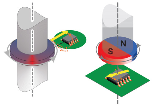
end-of-shaft angle measurement (right)
Measurement Errors
All Allegro angle sensor ICs are calibrated at final test in the factory using a homogenous magnetic field. This is done to minimize the native error of the sensor. However, especially in side-shaft applications, the magnetic field angle at the sensor transducer is not identical to the mechanical angle of the shaft that is to be measured. The main contributor to this difference is the shape of the magnetic field emitted from the encoder magnet.
Other sources of mismatch between mechanical and magnetic field angle are magnet misalignment, magnet imperfections, remaining sensor inaccuracy and drift, and the presence of ferromagnetic materials.
It can be concluded that all systems, and especially sideshaft-systems, suffer from a mismatch between the encoder angle and the measured angle. A typical transfer curve for a side-shaft application can be seen in Figure 2.
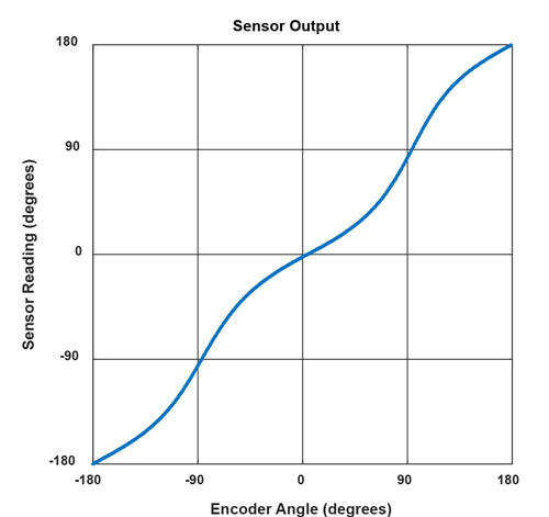
angle in a side-shaft setup
These measurement errors are called nonlinearities and can be compensated through a process called linearization.
Linearization
Some Allegro sensor ICs, such as the A1335, the AAS33001, and the AAS33051 have embedded logic that allows for the linearization of input data. This application note will explain how to use the linearization features of the AAS33001 and AAS33051. To simplify references to these parts, both will be referred to as AAS330x1 henceforth.
This application note will:
- Explain the fundamentals of linearization
- Explain the AAS330x1 linearization features
- Show how to process measured data to calculate correction data
- Explain how to calculate the sensor parameters
- Show the accuracy after linearization
Definitions
Encoder Angle
The angle reported by an accurate, high-resolution external encoder.
Sensor Angle
The angle reported by the angle sensor IC.
Angle Error
Angle error is the difference between the actual position of the magnet and the position of the magnet as measured by the angle sensor IC. This is calculated by subtracting the encoder angle from the sensor angle:
error = (α_sensor – α_encoder ) .
However, if the sensor angle is 359° and the encoder angle is 0°, the error should be –1° and not +359°. To wrap around any error outside of ±180°, the modulo operator can be used:
error = mod[(α_sensor – α_encoder) + 180,360] – 180.
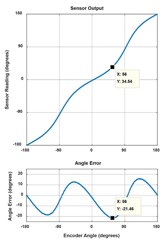
A sample plot of the angle error in a side-shaft application is given in Figure 3.
Maximum Absolute Angle Error
The maximum absolute angle error is the largest absolute difference between the actual position of the magnet and the position of the magnet as measured by the angle sensor IC over a full rotation.
In Figure 3, the maximum angle error is 21.46°, measured at an encoder angle of 56°.
Goal of Linearization
The goal of linearization is to determine, store, and apply a function that minimizes the measured sensor angle error as compared to the encoder angle value. This minimizes the difference between measured sensor angle and actual encoder angle.

angle to encoder angle
This goal can be achieved in different ways. Three common techniques will be detailed in this applications note.
The techniques presented depend on a single calibration phase (typically performed at the customer’s end-of-line test), after which a fixed correction function is applied.
Prerequisites to Linearization
Prerequisites to linearization using the techniques detailed here are the following:
- During production, known angles need to be applied to the sensor system.
- During production, sensor angles need to be read out.
- The system to be linearized needs a microcontroller, to which linearization information is written during the production process and which performs linearization in the application.
Limits to Linearization
Linearization using the methods described here has some limits:
- Sensor noise will not be corrected by linearization.
- Any drift of the sensor after calibration will not be corrected.
- Changes in the mechanical system after calibration will not be corrected by linearization. A common example is dynamic change of magnet position due to vibrations and torque.
- If the input positions during the calibration are not accurately recorded, the accuracy of the correction will be limited in the same way.
Linearization Method
1. Data Recording
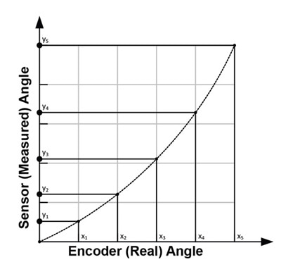
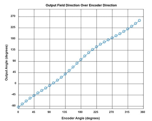
To generate the data needed for linearization, measure sensor output [y0 … yn] at known encoder angles [x0 … xn]. These encoder angles do not need to be equidistant, although it is common to use equidistant angles.
The recording of values is shown in Figure 5.
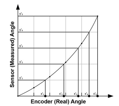
2. Coordinate Transformation to Sensor Angle
As the correction function has to work based on the sensor data, the recorded data points should be transformed into the sensor coordinate system. This means that instead of expressing the sensor angle as function of the real angle, it is required to express the real angle as function of the sensor angle. Therefore, sensor angles [y'0 … y'n] are chosen, for which corresponding encoder angles [x'0 … x'n] need to be determined. To do this, a fit needs to be applied through the data points. This can be done through spline interpolation, as shown in Figure 6.
3. Correction Curve Calculation
In order to create a function that converts the angle measured at the sensor into the encoder angle, correction values need to be calculated. These correction values are calculated as [c0 … cn] = [x'0 … x'n] – [y'0 … y'n].
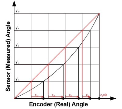
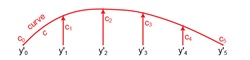
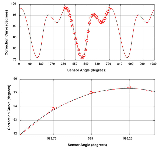
In the end, these values describe a correction curve, c, which gives the correction values as a function of the sensor angle. Figure 8 shows a plot of the curve c over sensor angle.
4. Correction Curve Application to Data
To apply the correction to a measured sensor data point, a correction value C for sensor data point Y needs to be calculated based on the correction curve c. This is graphically represented in Figure 9.
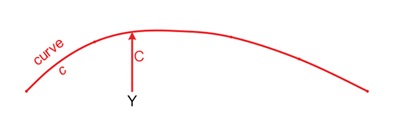
The correct angle value X is then determined as X = Y + C. This is graphically represented in Figure 10.
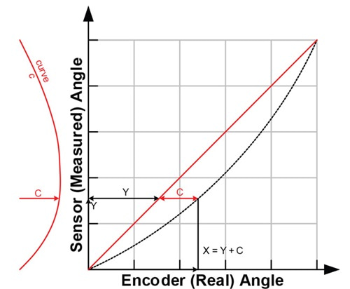
the correction curve
Correction Curve Determination
The implementations in this document were implemented in MathWorks MATLAB™. As this is commercial software, licensing costs apply to using it, which may hinder use in production environments. A free software alternative to MATLAB is GNU Octave, which is available under the GNU GPLv3 license free of charge.
All functions used in this document are supported by both MATLAB and GNU Octave.
Sensor Output Capture
Initial data on the sensor angular output must be captured by the user. This is done by setting certain known angles, referred to as encoder angles in this document. Then the sensor angles are recorded. The sensor angles are the angles measured by the sensor. The number of points recorded can be more or less than the number of linear correction points. Recording more points, if possible, is always better.
In general, recording at least 16 data points is enough for good correction performance in on-axis situations. In off-axis situations, at least 32 points are recommended.
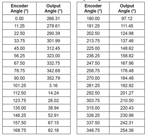
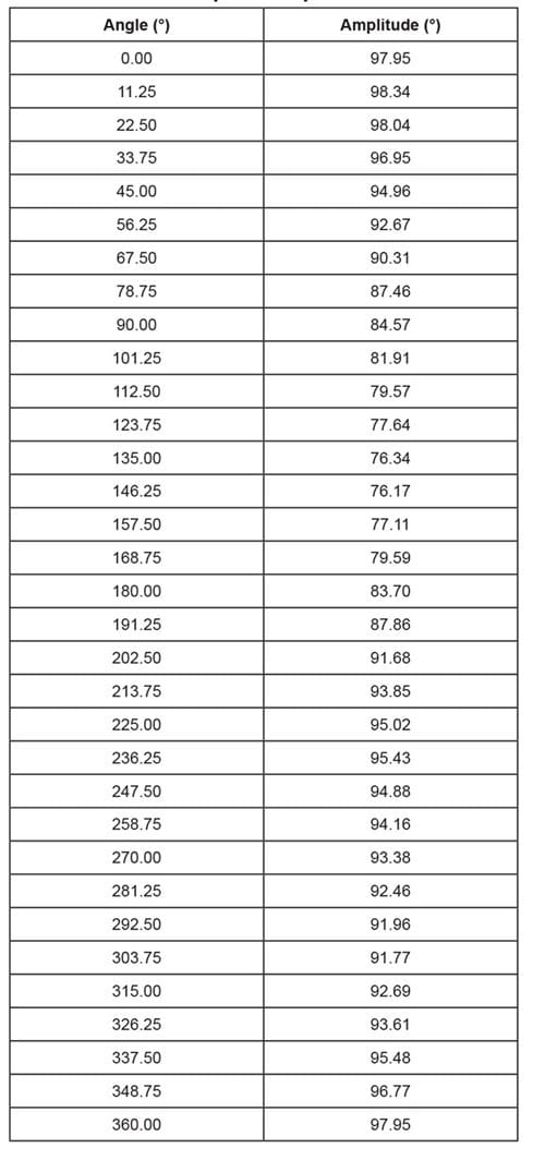
To apply piecewise linear correction with n segments (e.g. 32), recording at least n points will make good use of the available correction points. Recording about 2 × n points results in a nearly ideal performance. A real-life example of recorded points is given in Table 1.
Table 1: Recorded encoder and output angles
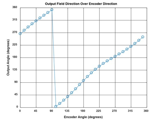
Sensor Output Overflow Removal
The jump in the sensor data around 100° input angle will cause difficulties in the next processing steps. It is removed by adding 360° to all values after the jump into negative direction. Also, the mean value of the data should be within ±180° to avoid other issues in later processing. This is achieved by the following lines:
The direction of the input data may need to be inverted. This is detected and performed by the following lines:%% pre-processing
% check if rising/falling continuously with maximum one overflow
if any(diff(sensor_data_2) == 0)
error('sensor data must be monotonously increasing or decreasing')
elseif sum(diff(sensor_data_2) < 0 ) <= 1
% rising angle data with zero or one overflows, overflow will be corrected
sensor_data_2 = sensor_data_2(:) + 360*cumsum([false; diff(sensor_data_2(:))
< 0 ]);
elseif sum(diff(sensor_data_2) > 0 ) <= 1
% falling angle data with zero or one overflows, overflow will be corrected
sensor_data_2 = sensor_data_2(:) - 360*cumsum([false; diff(sensor_data_2(:))
> 0 ]);
else
error('only one data overflow permitted')
end
The mean value of the data should be within ±180° to avoid other issues in later processing. This is achieved by the following lines:% invert angle direction, if needed
if all(diff(sensor_data_2) < 0 )
disp('inverting angle direction...')
sensor_data_2 = -sensor_data_2;
raw_direction = -1;
elseif all(diff(sensor_data_2) > 0 )
raw_direction = +1;
else
error('nonmonotonic angle changes detected')
end
The resulting values are shown in Table 2.% correctly wrap around sensor data
rollovercorrection = round((mean(sensor_data_2) - 180)/360) * 360;
sensor_data_2 = sensor_data_2 - rollovercorrection;
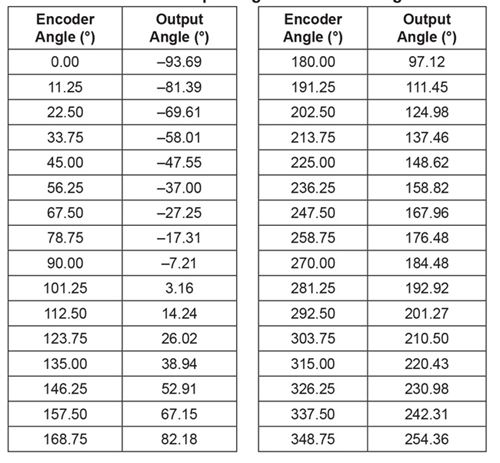
Table 2: Encoder and output angles after removing overflow
Data Replication
Eventually, correction data based on the sensor angles from 0° to 360° are needed. To avoid any edge effects, the sensor data will be replicated three times. This avoids edge effects in all cases by giving the possibility to always safely extract the values from sensor angle 360° to 720°.
%extend sensor data
sensor_data_ext = [sensor_data_2(:); sensor_data_2(:)+360; ...
sensor_data_2(:)+720];
%extend input data
angle_input_ext = [angle_input(:); angle_input(:)+360; ...
angle_input(:)+720];
Projection onto Sensor Data Grid
In the next step, the encoder angle inputs corresponding to sensor outputs between 360° and 720° are calculated (called “intermediategrid” in the code below). This is done with 4096 steps, as a high resolution for this intermediate step benefits the final output quality.
This step is graphically illustrated in Figure 13.%% use spline to move the data from an ordered input grid
% onto an ordered output grid:
ordered_output_grid = 0:(360/4096):(360-360/4096);
intermediategrid = ordered_output_grid + 360;
projection = spline(sensor_data_ext, angle_input_ext, ...
intermediategrid);
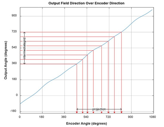
projection of a fixed-grid sensor angle (“intermediategrid”)
The correction curve can be seen below in Figure 14.% calculate the required correction of the data:
correction_curve = projection - intermediategrid;
correction_curve = correction_curve(:);
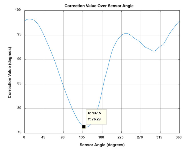
A brief check can be done to see that this curve is correct. In Table 1, it can be seen that for the sensor angle of 137.46°, the encoder angle is 213.75°. The correction curve of Figure 14 shows that at a sensor angle of 137.5°, a correction of +76.29° needs to be applied. As 137.46 + 76.26 = 213.72° ≅ 213.75°, the correction curve calculated is applicable.
At the next step, the correction curve needs to be stored in the AAS330x1. To explain how the sensor can apply correction, the concept of a piecewise linear correction will be explained first, then the AAS330x1 hardware capabilities, in order to determine the actual correction values.
Linear Interpolation
Concept
The correction curve can be approximated by a piecewise linear function. For this function, it is required to store support points as pairs of sensor coordinates and correction values.
In Figure 8, these pairs would be [(y'0, c0,) … (y'n, cn)].
Between the support points, linear interpolation is performed.
In angle sensor linearization applications, it is useful to use an equidistant grid of sensor angles. In this way, the sensor angle values [y'0 … y'n] do not need to be stored, and the implementation of the linear correction becomes easier. For example, it is possible to store 32 correction values, which will then be applied at sensor angles of 0°, 11.25°, 22.50°, etc.
The points to be stored can be determined by different criteria. The simplest way to determine them is by choosing points on the correction curve at said sensor angles, which will be referred to as “on-curve” linear interpolation. However, the points can also be optimized for a least-squares error of the stored correction curve. This will be referred to as “least-squares” linear interpolation.
Other optimization strategies are possible, but will not be described in this document.
The difference between on-curve and least-squares correction parameters for the curve from this example is seen in Figure 15.
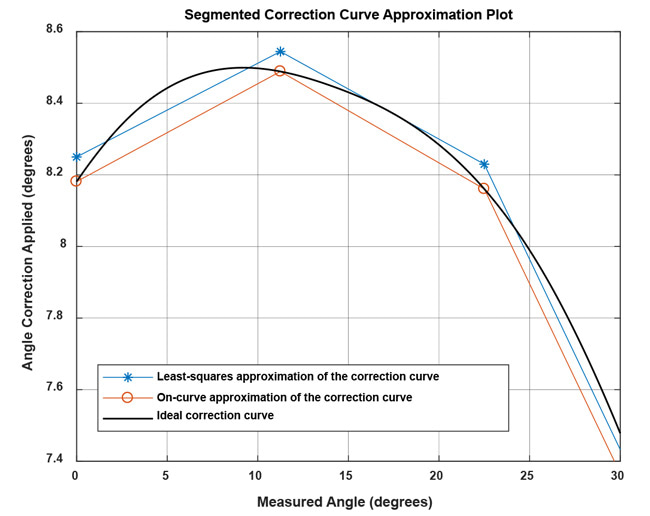
on-curve and least-squares method
The least-squares method reduces the amount of storage parameters needed by about 50% for the same maximum error and is less sensitive to single measurement outliers. Therefore, the leastsquares method will be used here to determine the linear interpolation support points.
Implementation
The correction curve needs to be approximated using a piecewise linear function. Because the support point should be chosen in a least-squares error fashion, the data before and after the support point also contributes in determining its final value.
This creates a problem for the first and last point. The first support point at 0° only has a correction curve to the right side of the point, so that the data close to 360° would not be taken into account. To avoid this problem, the correction curve will be repeated three times, and a piecewise linear least-squares approximation of that curve will be calculated. Then only the central part will be used to choose the parameters used. This concept is shown in Figure 16.
Fit Calculation
The code to replicate the correction curve and calculate the fit is given below:
%% piecewise linear approximation of the correction curve
lin_sup_nodes = 32;
% repeat the correction table three times to avoid
% corner effects on correction calculation.
triple_correction_curve = repmat(correction_curve,3,1);
triple_correction_curve(end+1) = triple_correction_curve(1);
% do the same with the angle input
triple_output_grid = 0:(360/4096):(3*360);
% calculate support points
XI_lin_triple = linspace(0,3*360,lin_sup_nodes*3+1);
YI_lin_triple = lsq_lut_piecewise( triple_output_grid(:), ...
triple_correction_curve, XI_lin_triple );
% use only the central points to calculate the correction:
YI_lin = YI_lin_triple(lin_sup_nodes+1 : 2*lin_sup_nodes+1);
XI_lin = linspace(0,360,lin_sup_nodes+1);
The lsq_lut_piecewise function is reprinted in Appendix A.
The list of correction parameters for 32-point linear interpolation is found below:
Table 3: Linear interpolation parameters
Note that a correction parameter for 360° is also shown, even though it is identical to the one for 0°. This was done to correct angles between 348.75° and 360° in the MATLAB script. The AAS330x1, however does not store the 360° value separately and uses the 0° value instead.
Figure 17 shows how the output error after linearization decreases as the number of linearization points increases. When 32 linearization points are used, the angular error becomes very small, showing that the number implemented in the AAS330x1 is sufficient.
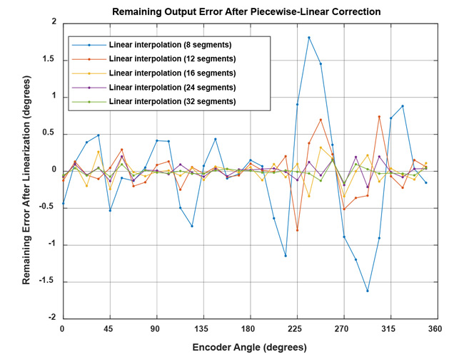
with an increasing amount of linear support nodes for
the example in this document
To understand how to determine the AAS330x1 programming parameters, the hardware capabilities of the AAS330x1 will be discussed first.
AAS330x1 Linearization Features
The AAS330x1 stores the correction curve using 32-segment piecewise linear approximation. The correction values are applied at equidistant sensor angles of 0°, 11.25°, 22.50°, …, 348.75°. Between these points, linear interpolation between the two adjacent supporting points is applied. The sensor performs the linearization in 188 ns, which is much faster than most microcontroller
implementations.
Hardware Features
The AAS330x1 contains an offset stage, a linearization stage, and a rotational direction inverter. As seen in Figure 18, the offset adjustment can be performed before or after linearization. In this document, it will be assumed that “zal” (Zero After Linearization) is set to ‘1’, which means that offset adjustment will be performed after linearization.
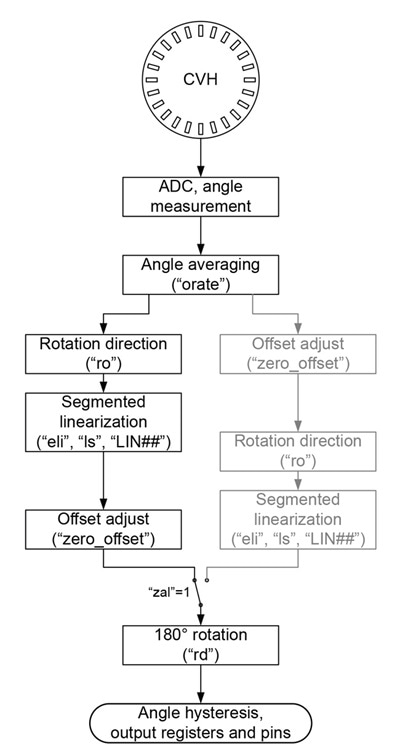
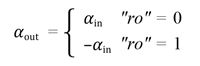
Rotation Direction
The rotation direction of the sensor can be inverted. If enabled, the angle value is inverted:
Segmented Linearization
Segmented linearization is enabled by setting “eli” to ‘1’. If enabled, the values “LIN##” are subtracted from the sensor output at an angle of (## / 32) × 360°. For example, the value for “LIN10” is applied at (10 / 32) × 360° = 112.5°. Values between these angles are linearly interpolated between the adjacent support points. For example, the correction value at 115° will be determined based on the values of “LIN10” and “LIN11”.
The LIN fields are 12-bit signed values and written in 2’s complement. The resolution depends on the bit “ls” and is 22.5° / 2048 LSB for “ls” = ’0’ and 45° / 2048 LSB for “ls” = ’1’. Because they are subtracted from the angle, negative values in the LIN fields increase the angle output of the sensor. This is detailed in the following table:
Table 4: Recorded encoder and output angles for sensor_data
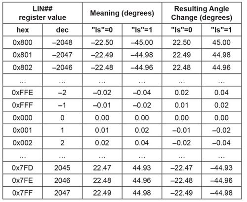
For example, if the value for LIN00 is set to 0xD0F, this represents a decimal value of 3343 – 212 = –753. If “ls” is set to ‘0’, this equals an angle value of 22.5° / 2048 LSB × ( 753 LSB) = –8.27°. This value will be subtracted from the measured angle, so for an input of 0°, the linearization block will output 0° – (–8.27°) = +8.27°.
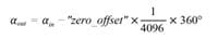
Offset Adjustment
The offset adjustment stage of the sensor aligns the zero values of the sensor to that of the external encoder. It is controlled by the EEPROM field “zero_offset”, which allows writing a 12-bit value. This unsigned value represents an angle between 0° and (4095 / 4096) × 360°, which is subtracted from the original angle value.
180° Rotation
In a final processing step, the sensor output can be rotated by 180°:
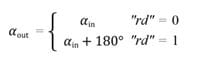
This function can be performed equally well by the offset stage, so that the die rotation function in this document will not be used.
Parameter Calculation
Knowing how the sensor works, the correction curve described in Table 3 can now be represented in terms of sensor parameters. This is done by first using the information on rotation direction and offset determined from the data. Then the linearization parameter scale can be selected, and the full linearization value table can be determined.
At the end of this code, the function cell2csv is used to write a CSV table that can be imported by the Allegro AAS33001 / AAS33051 Samples Programmer. The function cell2csv is reprinted in Appendix B. Many similar functions are in circulation, but the one provided should suffice. The resulting table for our example is the following:%% calculate AAS330x1 parameters
% "zal": zero-after-linearization is always zero
disp(['*** AAS330x1 "zal" parameter in EEPROM should be set to 1']);
% "eli": enable linearization is always one
disp(['*** AAS330x1 "eli" parameter in EEPROM should be set to 1']);
% "ro": Die rotation should be enabled if direction of sensor angles was
decreasing.
if (raw_direction == -1)
sensor_EEPROM_val_ro = 1;
else
sensor_EEPROM_val_ro = 0;
end
disp(['*** AAS330x1 "ro" parameter in EEPROM should be set to '
num2str(sensor_EEPROM_val_ro)]);
% "zero_offset": Offset should set as average of min and max offset.
% This will make best use of the range of +/-45 degrees that the
linearization parameters have.
zero_offset = mean([min(YI_lin) max(YI_lin)]);
% sensor offset is subtracted from angle data. If sensor direction is
inverted, this takes place before angle inversion,
% so that the sensor offset sign must be inverted in that case
sensor_EEPROM_val_zero_offset = uint16(mod(round(-zero_
offset/360*4096),4096));
disp(['*** AAS330x1 "zero_offset" parameter in EEPROM should be set to '
num2str(sensor_EEPROM_val_zero_offset)]);
% "ls": Linearization scale must be set depending on the maximum parameter
values.
linearization_range_small = 22.5 * (2047/2048);
linearization_range_large = 45.0 * (2047/2048);
if round(max(abs(YI_lin - zero_offset))) < linearization_range_small
sensor_EEPROM_val_ls = uint16(0);
elseif round(max(abs(YI_lin - zero_offset))) < linearization_range_large
sensor_EEPROM_val_ls = uint16(1);
else
error('Linearization parameters outside of +/-45° range;
linearization not possible')
end
disp(['*** AAS330x1 "ls" parameter in EEPROM should be set to '
num2str(sensor_EEPROM_val_ls)]);
% "LIN_##" parameters
if (sensor_EEPROM_val_ls == 0) % small range of +/- 22.5°
sensor_EEPROM_val_LIN = int16(round((zero_offset-YI_lin(1:lin_sup_
nodes))/22.5*2048));
else % larger range of +/- 45.0°
sensor_EEPROM_val_LIN = int16(round((zero_offset-YI_lin(1:lin_sup_
nodes))/45.0*2048));
end
disp(['*** AAS330x1 "LIN_##" parameters in EEPROM should be set to the
following values:']);
disp(num2str(sensor_EEPROM_val_LIN));
%% write csv table for Allegro AAS330x1 Samples Programmer
EEPtable = cell(38,2);
EEPtable(1,1:2) = {'EEPROM',''};
EEPtable(2,1:2) = {'zal',1};
EEPtable(3,1:2) = {'eli',1};
EEPtable(4,1:2) = {'ro',sensor_EEPROM_val_ro};
EEPtable(5,1:2) = {'zero_offset',sensor_EEPROM_val_zero_offset};
EEPtable(6,1:2) = {'ls',sensor_EEPROM_val_ls};
for i = 1:32
EEPtable{6+i,1} = num2str(['Linearization Error Segment ' num2str(i-
1,'%02d')]);
EEPtable{6+i,2} = num2str(sensor_EEPROM_val_LIN(i));
end
cell2csv('EEP_table.csv',EEPtable);
EEPROM,
zal,1
eli,1
ro,0
zero_offset,3103
ls,0
Linearization Error Segment 00,-973
Linearization Error Segment 01,-1009
Linearization Error Segment 02,-981
Linearization Error Segment 03,-881
Linearization Error Segment 04,-701
Linearization Error Segment 05,-492
Linearization Error Segment 06,-278
Linearization Error Segment 07,-18
Linearization Error Segment 08,245
Linearization Error Segment 09,487
Linearization Error Segment 10,701
Linearization Error Segment 11,875
Linearization Error Segment 12,994
Linearization Error Segment 13,1009
Linearization Error Segment 14,924
Linearization Error Segment 15,699
Linearization Error Segment 16,323
Linearization Error Segment 17,-54
Linearization Error Segment 18,-402
Linearization Error Segment 19,-600
Linearization Error Segment 20,-707
Linearization Error Segment 21,-744
Linearization Error Segment 22,-694
Linearization Error Segment 23,-627
Linearization Error Segment 24,-558
Linearization Error Segment 25,-474
Linearization Error Segment 26,-428
Linearization Error Segment 27,-411
Linearization Error Segment 28,-494
Linearization Error Segment 29,-578
Linearization Error Segment 30,-748
Linearization Error Segment 31,-865
Performance Estimation
The accuracy after linearization with the parameters used can be estimated in simulation. For that, the linearization parameters that were determined need to be applied in simulation, together with the optional direction inversion:
Figure 19 shows the expected angle error after linearization in the AAS330x1:%% perform linearization in MATLAB
restored_linear_signal = mod(raw_direction*sensor_data(:) + ...
interp1(XI_lin,YI_lin,mod(raw_direction*sensor_data(:),360),'linear'),360);
%% plot the remaining error after linearization in MATLAB
figure;
plot(angle_input(:),mod(180+restored_linear_signal(:)-angle_input(:),360)-
180,'.-');
grid on;legend('Linear interpolation (32 segments)');
xlim([0 360]); ylim([-1 1]);
xlabel('Measured angle [deg]');
ylabel('Expected error after linearization [deg]');
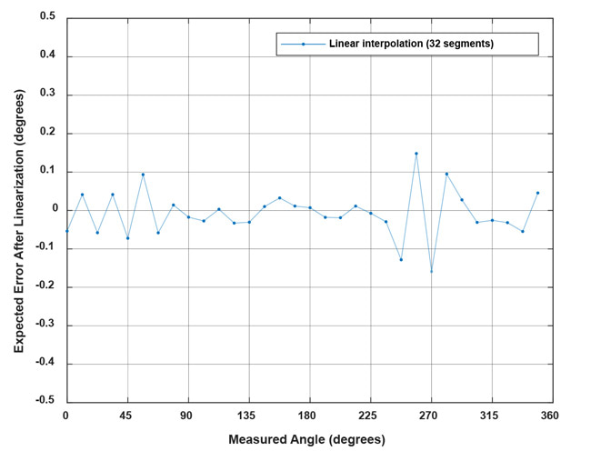
with AAS330x1 as described in this document,
for the example from this document
Conclusion
This document explains the theory behind linearization in general and describes how linear approximation of the correction can be done.
The AAS33001 and AAS33051 allow for segmented linearization. This linearization method is performed in under 0.2 μs by the sensors, and achieves very good accuracy with 32 segments.
Using this document, any user should be able to determine the best linearization parameters for the AAS33001 and AAS33051.
Contact an Allegro representative for any remaining questions or support.
APPENDIX A: FUNCTION LSQ_LUT_PIECEWISE
From https://uk.mathworks.com/matlabcentral/fileexchange/40913-piecewise-linear-least-square-fit.
Copyright (c) 2013, Guido Albertin
All rights reserved.
Redistribution and use in source and binary forms, with or without modification, are permitted provided that the following conditions are met:
* Redistributions of source code must retain the above copyright notice, this list of conditions and the following disclaimer.
* Redistributions in binary form must reproduce the above copyright notice, this list of conditions and the following disclaimer in the documentation and/or other materials provided with the distribution
THIS SOFTWARE IS PROVIDED BY THE COPYRIGHT HOLDERS AND CONTRIBUTORS “AS IS” AND ANY EXPRESS OR IMPLIED WARRANTIES, INCLUDING, BUT NOT LIMITED TO, THE IMPLIED WARRANTIES OF MERCHANTABILITY AND FITNESS FOR A PARTICULAR PURPOSE ARE DISCLAIMED. IN NO EVENT SHALL THE COPYRIGHT OWNER OR CONTRIBUTORS BE LIABLE FOR ANY DIRECT, INDIRECT, INCIDENTAL, SPECIAL, EXEMPLARY, OR CONSEQUENTIAL DAMAGES (INCLUDING, BUT NOT LIMITED TO, PROCUREMENT OF SUBSTITUTE GOODS OR SERVICES; LOSS OF USE, DATA, OR PROFITS; OR BUSINESS INTERRUPTION) HOWEVER CAUSED AND ON ANY THEORY OF LIABILITY, WHETHER IN CONTRACT, STRICT LIABILITY, OR TORT (INCLUDING NEGLIGENCE OR OTHERWISE) ARISING IN ANY WAY OUT OF THE USE OF THIS SOFTWARE, EVEN IF ADVISED OF THE POSSIBILITY OF SUCH DAMAGE.
function [ YI ] = lsq_lut_piecewise( x, y, XI )
% LSQ_LUT_PIECEWISE Piecewise linear interpolation for 1-D interpolation (table lookup)
% YI = lsq_lut_piecewise( x, y, XI ) obtain optimal (least-square sense)
% vector to be used with linear interpolation routine.
% The target is finding Y given X the minimization of function
% f = |y-interp1(XI,YI,x)|^2
%
% INPUT
% x measured data vector
% y measured data vector
% XI break points of 1-D table
%
% OUTPUT
% YI interpolation points of 1-D table
% y = interp1(XI,YI,x)
%
if size(x,2) ~= 1
error('Vector x must have dimension n x 1.');
elseif size(y,2) ~= 1
error('Vector y must have dimension n x 1.');
elseif size(x,1) ~= size(x,1)
error('Vector x and y must have dimension n x 1.');
end
% matrix defined by x measurements
A = sparse([]);
% vector for y measurements
Y = [];
for j=2:length(XI)
% get index of points in bin [XI(j-1) XI(j)]
ix = x>=XI(j-1) & x<XI(j);
% check if we have data points in bin
if ~any(ix)
warning(sprintf('Bin [%f %f] has no data points, check estimation.
Please re-define X vector accordingly.',XI(j-1),XI(j)));
end
% get x and y data subset
x_ = x(ix);
y_ = y(ix);
% create temporary matrix to be added to A
tmp = [(( -x_+XI(j-1) ) / ( XI(j)-XI(j-1) ) + 1) (( x_-XI(j-1) ) / ( XI(j)-XI(j-1) ))];
% build matrix of measurement with constraints
[m1,n1]=size(A);
[m2,n2]=size(tmp);
A = [[A zeros(m1,n2-1)];[zeros(m2,n1-1) tmp]];
% concatenate y measurements of bin
Y = [Y; y_];
end
% obtain least-squares Y estimation
YI=A\Y;
APPENDIX B: FUNCTION CELL2CSV
Based on https://uk.mathworks.com/matlabcentral/fileexchange/7601-cell2csv.
function cell2csv(filename,cellArray,delimiter)
% Writes cell array content into a *.csv file.
%
% CELL2CSV(filename,cellArray,delimiter)
%
% filename = Name of the file to save. [ i.e. 'text.csv' ]
% cellarray = Name of the Cell Array where the data is in
% delimiter = Seperating sign, normally:',' (it's default)
%
% by Sylvain Fiedler, KA, 2004
% modified by Rob Kohr, Rutgers, 2005 - changed to english and fixed delimiter
% modified by Dominik Geisler, Allegro MicroSystems, 2018 - removed 'eval' function
if nargin<3
delimiter = ',';
end
file = fopen(filename,'w');
for z=1:size(cellArray,1)
for s=1:size(cellArray,2)
var = cellArray{z,s};
if size(var,1) == 0
var = '';
end
if isnumeric(var) == 1
var = num2str(var);
end
fprintf(file,var);
if s ~= size(cellArray,2)
fprintf(file,[delimiter]);
end
end
fprintf(file,'\n');
end
fclose(file);
APPENDIX C: FUNCTION ENTIRE SCRIPT USED IN THIS APPLICATION NOTE
Copyright (c) 2018, Dominik Geisler, Allegro MicroSystems Germany GmbH
All rights reserved.
Redistribution and use in source and binary forms, with or without modification, are permitted provided that the following conditions are met:
* Redistributions of source code must retain the above copyright notice, this list of conditions and the following disclaimer.
* Redistributions in binary form must reproduce the above copyright notice, this list of conditions and the following disclaimer in the documentation and/or other materials provided with the distribution
THIS SOFTWARE IS PROVIDED BY THE COPYRIGHT HOLDERS AND CONTRIBUTORS “AS IS” AND ANY EXPRESS OR IMPLIED WARRANTIES, INCLUDING, BUT NOT LIMITED TO, THE IMPLIED WARRANTIES OF MERCHANTABILITY AND FITNESS FOR A PARTICULAR PURPOSE ARE DISCLAIMED. IN NO EVENT SHALL THE COPYRIGHT OWNER OR CONTRIBUTORS BE LIABLE FOR ANY DIRECT, INDIRECT, INCIDENTAL, SPECIAL, EXEMPLARY, OR CONSEQUENTIAL DAMAGES (INCLUDING, BUT NOT LIMITED TO, PROCUREMENT OF SUBSTITUTE GOODS OR SERVICES; LOSS OF USE, DATA, OR PROFITS; OR BUSINESS INTERRUPTION) HOWEVER CAUSED AND ON ANY THEORY OF LIABILITY, WHETHER IN CONTRACT, STRICT LIABILITY, OR TORT (INCLUDING NEGLIGENCE OR OTHERWISE) ARISING IN ANY WAY OUT OF THE USE OF THIS SOFTWARE, EVEN IF ADVISED OF THE POSSIBILITY OF SUCH DAMAGE.
%% sensor data definition
angle_input = [0:11.25:348.75];
sensor_data = [266.31 278.61 290.39 301.99 312.45 323.00 332.75 342.69 352.79 3.16 14.24 26.02 38.94 52.91 67.15 82.18 97.12 111.45 124.98 137.46 148.62 158.82
167.96 176.48 184.48 192.92 201.27 210.50 220.43 230.98 242.31 254.36];
%% Check rising reference angle
if any(angle_input<0) || any(angle_input>360) || any(diff(angle_input)<=0)
error('reference angle must be monotonuously rising between 0 and 360');
end
%% Check correct sensor angle range
if any(sensor_data<0) || any(sensor_data>360)
error('sensor angle must be between 0 and 360');
end
%% pre-processing
sensor_data_2 = sensor_data(:);
% check if rising/falling continuously with maximum one overflow
if any(diff(sensor_data_2) == 0)
error('sensor data must be monotonously increasing or decreasing')
elseif sum(diff(sensor_data_2) < 0 ) <= 1
% rising angle data with zero or one overflows, overflow will be corrected
sensor_data_2 = sensor_data_2(:) + 360*cumsum([false; diff(sensor_data_2(:)) < 0 ]);
elseif sum(diff(sensor_data_2) > 0 ) <= 1
% falling angle data with zero or one overflows, overflow will be corrected
sensor_data_2 = sensor_data_2(:) - 360*cumsum([false; diff(sensor_data_2(:)) > 0 ]);
else
error('only one data overflow permitted')
end
    % invert angle direction, if needed

if all(diff(sensor_data_2) < 0 )

disp('inverting angle direction...')

sensor_data_2 = -sensor_data_2;

raw_direction = -1;

elseif all(diff(sensor_data_2) > 0 )

raw_direction = +1;

else

error('nonmonotonic angle changes detected')

end
    % correctly wrap around sensor data

rollovercorrection = round((mean(sensor_data_2) - 180)/360) * 360;

sensor_data_2 = sensor_data_2 - rollovercorrection;
%extend sensor data
sensor_data_ext = [sensor_data_2(:); sensor_data_2(:)+360; ...

sensor_data_2(:)+720];


%extend input data

angle_input_ext = [angle_input(:); angle_input(:)+360; ...

angle_input(:)+720];
%% plot magnet measurements after preprocessing finished
figure;plot([angle_input(:)],[sensor_data_2(:)],'o-');
xlabel('Encoder angle [deg]');
ylabel('Output angle [deg]');
grid on;
xlim([0 360]);
if (raw_direction == +1)
title('Output field direction over encoder direction');
else
title('Output field direction over encoder direction after direction inversion');
end
%% use spline to move the data from an ordered input grid

% onto an ordered output grid:

ordered_output_grid = 0:(360/4096):(360-360/4096);

intermediategrid = ordered_output_grid + 360;

projection = spline(sensor_data_ext, angle_input_ext, ...

intermediategrid);
% calculate the required correction of the data:

correction_curve = projection - intermediategrid;

correction_curve = correction_curve(:);
%% piecewise linear approximation of the correction curve

lin_sup_nodes = 32;

% repeat the correction table three times to avoid

% corner effects on correction calculation.

triple_correction_curve = repmat(correction_curve,3,1);

triple_correction_curve(end+1) = triple_correction_curve(1);

% do the same with the angle input

triple_output_grid = 0:(360/4096):(3*360);

% calculate support points

XI_lin_triple = linspace(0,3*360,lin_sup_nodes*3+1);

YI_lin_triple = lsq_lut_piecewise( triple_output_grid(:), ...

triple_correction_curve, XI_lin_triple );

% use only the central points to calculate the correction:

YI_lin = YI_lin_triple(lin_sup_nodes+1 : 2*lin_sup_nodes+1);

XI_lin = linspace(0,360,lin_sup_nodes+1);
%% calculate AAS330x1 parameters
% "zal": zero-after-linearization is always zero
disp(['*** AAS330x1 "zal" parameter in EEPROM should be set to 1']);
% "eli": enable linearization is always one
disp(['*** AAS330x1 "eli" parameter in EEPROM should be set to 1']);
% "ro": Die rotation should be enabled if direction of sensor angles was decreasing.
if (raw_direction == -1)
sensor_EEPROM_val_ro = 1;
else
sensor_EEPROM_val_ro = 0;
end
disp(['*** AAS330x1 "ro" parameter in EEPROM should be set to ' num2str(sensor_EEPROM_val_ro)]);
% "zero_offset": Offset should set as average of min and max offset.
% This will make best use of the range of +/-45 degrees that the linearization parameters have.
zero_offset = mean([min(YI_lin) max(YI_lin)]);
% sensor offset is subtracted from angle data. If sensor direction is inverted, this takes place before angle inversion,
% so that the sensor offset sign must be inverted in that case
sensor_EEPROM_val_zero_offset = uint16(mod(round(-zero_offset/360*4096),4096));
disp(['*** AAS330x1 "zero_offset" parameter in EEPROM should be set to ' num2str(sensor_EEPROM_val_zero_offset)]);
% "ls": Linearization scale must be set depending on the maximum parameter values.
linearization_range_small = 22.5 * (2047/2048);
linearization_range_large = 45.0 * (2047/2048);
if round(max(abs(YI_lin - zero_offset))) < linearization_range_small
sensor_EEPROM_val_ls = uint16(0);
elseif round(max(abs(YI_lin - zero_offset))) < linearization_range_large
sensor_EEPROM_val_ls = uint16(1);
else
error('Linearization parameters outside of +/-45° range; linearization not possible')
end
disp(['*** AAS330x1 "ls" parameter in EEPROM should be set to ' num2str(sensor_EEPROM_val_ls)]);
% "LIN_##" parameters
if (sensor_EEPROM_val_ls == 0) % small range of +/- 22.5°
sensor_EEPROM_val_LIN = int16(round((zero_offset-YI_lin(1:lin_sup_nodes))/22.5*2048));
else % larger range of +/- 45.0°
sensor_EEPROM_val_LIN = int16(round((zero_offset-YI_lin(1:lin_sup_nodes))/45.0*2048));
end
disp(['*** AAS330x1 "LIN_##" parameters in EEPROM should be set to the following values:']);
disp(num2str(sensor_EEPROM_val_LIN));
%% write csv table for Allegro AAS330x1 Samples Programmer
EEPtable = cell(38,2);
EEPtable(1,1:2) = {'EEPROM',''};
EEPtable(2,1:2) = {'zal',1};
EEPtable(3,1:2) = {'eli',1};
EEPtable(4,1:2) = {'ro',sensor_EEPROM_val_ro};
EEPtable(5,1:2) = {'zero_offset',sensor_EEPROM_val_zero_offset};
EEPtable(6,1:2) = {'ls',sensor_EEPROM_val_ls};
for i = 1:32
EEPtable{6+i,1} = num2str(['Linearization Error Segment ' num2str(i-1,'%02d')]);
EEPtable{6+i,2} = num2str(sensor_EEPROM_val_LIN(i));
end
cell2csv('EEP_table.csv',EEPtable);
%% perform linearization in Matlab
restored_linear_signal = mod(raw_direction*sensor_data(:) + ...
interp1(XI_lin,YI_lin,mod(raw_direction*sensor_data(:),360),'linear'),360);
%% plot the remaining error after linearization in Matlab
figure;
plot(angle_input(:),mod(180+restored_linear_signal(:)-angle_input(:),360)-180,'.-');
grid on;legend('Linear interpolation (32 segments)');
xlim([0 360]); ylim([-1 1]);xlabel('Measured angle [deg]');
ylabel('Expected error after linearization [deg]');
Copyright ©2018, Allegro MicroSystems, LLC
The information contained in this document does not constitute any representation, warranty, assurance, guaranty, or inducement by Allegro to the customer with respect to the subject matter of this document. The information being provided does not guarantee that a process based on this information will be reliable, or that Allegro has explored all of the possible failure modes. It is the customer’s responsibility to do sufficient qualification testing of the final product to insure that it is reliable and meets all design requirements.