Range-Walk Correction Using Time Over Threshold

Introduction

Time-of-flight lidar systems measure pulse-return time of arrival based on the transition of the pulse return’s rising edge through a detection threshold. These systems are subject to systematic range error, termed range walk, caused by variations in pulse-return amplitude: For two otherwise identical pulse returns of differing amplitude that are both strong enough to exceed a fixed detection threshold, the rising edge of the weaker pulse return will cross the threshold at a time closer to the center of the pulse than the rising edge of the stronger pulse return.

Because range walk is a systematic error and because range walk is a monotonic function of pulse-return amplitude, it can be corrected based on pulse-return-amplitude measurements.

However, in most lidar applications, the dynamic range of the pulse-return amplitudes exceeds the dynamic range of the electronics of the photoreceivers, leading to signal saturation.

A simple alternative is to use time-over-threshold measurements. Time over threshold—the elapsed time between passage of the rising and falling edges of a pulse return through a detection threshold—is monotonically related to pulse amplitude but simpler to measure.

This paper shows that a lookup table or polynomial correction based on time-over-threshold measurements can be used to reduce the range walk of an avalanche photodiode-based lidar system to within ±0.2 meters, at all ranges, over a pulse-return dynamic range of greater than 90 dB.

Background

Time-of-flight lidar systems measure the distance to a target based on the round-trip travel time of nanosecond-scale laser pulses transmitted by the lidar and reflected back to the lidar by the target (Figure 1).

 

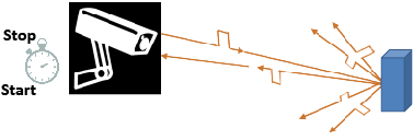
Figure 1: Basics of time-of-flight lidar: The lidar clocks the time of flight, which is the interval between when it detects transmission of the outgoing laser pulse and reception of the reflected target return. The time of flight is then converted to a range using the speed of light.

An avalanche-photodiode (APD) -based lidar photoreceiver circuit is diagrammed in Figure 2. In this style of receiver, the APD converts the optical signal into a photocurrent pulse and a low-noise transimpedance amplifier (TIA) converts the current pulse into a voltage pulse. A threshold comparator then converts the analog voltage pulse into a digital signal that can be timed by a time-to-digital converter (TDC).

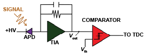
Figure 2: Block diagram of an APD-based lidar photoreceiver. (+HV is the APD high-voltage reverse bias, V_out is the analog voltage signal output by the TIA, V_th is the detection threshold; V_out is compared to V_th.)

In an ideal case, the physical time of flight (τ) is the time interval between the center of the transmitted laser pulse (T₀) and the center of its target reflection (T_stop):

Equation 1:

τ = T_stop – T₀ [s].

Target range (R, in meters) is calculated from τ and the speed of light in air, which is the same as the speed of light in vacuum (c, in m/s) to within about one part per 10,000:

Equation 2:

Errors in Time-of-Flight Methods

In contrast to the ideal case, ranging measurements are subject to systematic errors, which can be corrected by calibration, and random errors, which cannot. Systematic errors lead to loss of range accuracy and random errors lead to loss of range precision.^[1]

Random (Uncorrectable) Errors

In contrast to the systematic error in τ_offset, random processes in both APD and TIA cause the value of τ_offset, measured from a target at constant range, to fluctuate over an ensemble of identically prepared measurements, even when the mean pulse amplitudes and detection thresholds are constant. Because the magnitude of the fluctuation is random for each measurement, it cannot be removed by calibration.

The random timing error originates from high-frequency amplitude noise from the APD and the TIA superimposed on the rising signal pulse into the lidar comparator, as sketched in Figure 3, left: For any given measurement, an upward fluctuation of the noisy signal into the comparator advances the time that the signal crosses the detection threshold, and a downward fluctuation delays the time that the pulse is detected. Over an ensemble of identically prepared measurements, the magnitude of the high-frequency amplitude noise is quantified by the standard deviation of the signal amplitude at the average time of threshold-crossing (σ_n). The average slope of the rising signal at the threshold-crossing time (dV/dt) transforms the high-frequency amplitude noise into timing jitter (σ_t), which is the standard deviation of the pulse-detection time over an ensemble of measurements. 

Jitter cannot be removed by calibration because the magnitude of the noise fluctuations is random for each measurement.

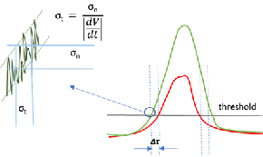
Figure 3: Jitter (σ_t ), diagrammed to the left, is a random error, so it is not correctable. Jitter results from the high-frequency amplitude noise (σ_n) superimposed on the signal pulse. The slope of the rising mean signal pulse (dV/dt) at the threshold-crossing transforms σ_n into σ_t . Unlike jitter, the range-walk timing offset of a single pulse (Δτ; diagrammed to the right), is a systematic error resulting from the variation of threshold-crossing time with signal-pulse amplitude, so it is correctable.

Obviously, measurements of both high accuracy and precision are desired. In practice, lidar systems are engineered to minimize the random errors responsible for imprecision, then calibrated to remove the systematic errors responsible for inaccuracy. Methods to remove systematic range-walk error are described next.

Systematic (Correctable) Errors

One type of systematic error is easily understood based on Equation 2, which assumes that the speed of light in the optical path between the lidar system and the target is exactly equal to the speed of light in vacuum. This assumption introduces a systematic error that can be removed if the average group refractive index (n) in the path—which depends on environmental factors such as atmospheric pressure, temperature, and humidity—is known:

Equation 3:

Range walk is another type of systematic error that depends on the pulse-return amplitude. The term range walk is used for this amplitude-dependent error because, for a given lidar system and target, pulse-return amplitude varies as exp(–2σR) R^–2 for area targets that are larger than the projected laser spot and as exp(–2σR) R^–4 for area targets that are smaller than the projected laser spot, where σ is the atmospheric attenuation coefficient in m–1. Thus, this type of range error is itself a function of range.^[2]

Errors in range accuracy due to range walk result from the pulse timing diagrammed in Figure 4. Whereas τ is the time interval between the centers of the transmitted (start) and reflected (stop) pulses (T₀ and T_stop), for a photoreceiver circuit such as that diagrammed in Figure 2, pulses are timed based on when the leading edges transition through the detection threshold (at times T_0,th and T_stop,th). The offsets ΔT₀ and ΔT_stop between the centers of the respective pulses and when the pulses are detected by the receiver circuit combine to result in an offset time-of-flight measurement (τ_offset). The timing offset depends on the pulse amplitude and the detection threshold in a systematic way, so the resulting range error is also systematic, and therefore correctable.

 

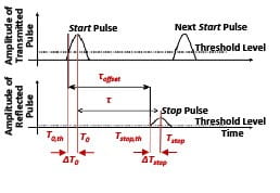
Figure 4: Lidar systems that use leading-edge detectors measure an offset time of flight (τ_offset): The physical time of flight (τ) is offset by time intervals that depend on the amplitudes of the transmitted and reflected pulses. These time intervals, ΔT₀ and ΔT_stop, also depend on the detection thresholds used to time them.

The physical time of flight (τ) is related to the measured offset time of flight (τoffset) by:

Equation 4:

τ = τ_offset + Δτ [s],

where the total systematic error Δτ is:

Equation 5:

Δτ = ΔT_stop – ΔT₀ [s].

The range walk associated with either a start (T₀) or stop (T_stop) pulse is illustrated in Figure 3, right, where two pulses of the same shape but different amplitude, with peaks occurring at the same time, are superimposed. As with timing jitter, a shift upward in the signal level causes the leading edge of a pulse to cross the detection threshold earlier. However, unlike jitter, the upward shift is a consequence of the laser pulse amplitude and not a random fluctuation, so the timing offset is systematic. Similarly, for return signals of a constant amplitude, varying the threshold from low levels to high levels, causes a systematic range-walk error, which decreases as the threshold approaches the pulse amplitude.

Correcting Systematic Range-Walk Errors

In practical lidar applications, the change in the signal amplitude relative to the detection-threshold level, as a function of the target range, target size, and target reflectivity, will lead to systematic range errors.

For lidar systems that use leading-edge pulse detection, the timing offsets responsible for range walk are proportional to pulse amplitude and are deterministic—meaning they can be removed by calibration if the pulse amplitude can be measured and if the quantitative relationship between the pulse amplitude and the timing offset is known.

A model of the signal amplitude of laser pulse echoes from targets at ranges from 25 m to 25 km returned to the input of a 21 mm aperture lidar system is shown in Figure 5. From the time the laser pulse leaves the transmitter, until the time the pulse returns from the nearest target (0 meters) and the most distant detectable target (roughly 25 km)—signal amplitude varies significantly. Within the full range of sensitivity of the example lidar system presented here, the signal amplitude varies by greater than 90 dB.

 

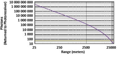
Figure 5: The signal-return amplitude calculated varies by about 90 dB for target ranges between 0 m and 25 km.

Ideally, the aperture-referred detection-threshold level would be kept at a fixed proportion to the signal amplitude, so that the ratio of the pulse amplitude to the threshold level would be the same for the outgoing pulse at the start time (T₀) as the ratio of the pulse amplitude to the threshold level at stop time (T_stop).

Range walk for various-amplitude single-return laser pulses (either T₀ or T_stop) is illustrated in the Figure 6, top, where 7 ns full-width at half maximum (FWHM) Gaussian pulses of peak amplitude varying between 0.1 and 1 arbitrary units (AU) are overlaid. For the sake of simplicity, here it is assumed that the APD and TIA have infinite bandwidth and are capable of reproducing the ideal Gaussian laser pulse. As the figure shows, for a detection threshold fixed at 0.1 AU, up to 7 ns of range-walk error may result.

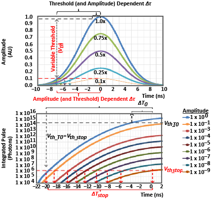
Figure 6: Even a 10 dB variation in signal amplitude can result in 7 ns of timing offset for a 7 ns FWHM Gaussian pulse if a fixed detection threshold is used (top). A time-variable threshold can, in principle, correct up to 20 ns of offset in this scenario (bottom).

An example for a wider range of signal amplitudes is shown in Figure 6, bottom. In this example, it is assumed that the TIA has an ability to integrate the signal pulse. In this example, which has a signal dynamic range closer to that modeled in Figure 5, the range-walk error can be as much as 20 ns for large signal returns detected with a photoreceiver operated at a low threshold level. According to Equation 3, a 20 ns timing error would result in a 3-meter range-accuracy error. For fixed-threshold detection systems, such errors are unavoidable because the threshold detector is used to sense both the outgoing laser pulse and the returns from the most distant detectable targets.

There are several ways to decrease systematic range errors in lidar systems. These include operational methods, such as time-variable threshold, and calibration methods, such as time over threshold; these methods can be used individually or together to improve range accuracy.

Time-Variable Threshold

Because the signal-return amplitude varies with range in a systematic way that is proportional with range between exp(–2σR) R^–4 and exp(–2σR) R^–2, range-walk error is itself a function of range. Thus, it is possible—in principle—to vary the detection threshold with time in such a way as to track the general trend in signal-return amplitude, so that range-walk error is reduced.

In a lidar system configured for operation with time-variable-threshold, the detection threshold (V_th) is adjusted over the course of the range measurement from an initial high value (V_{th_T0}) to the lowest value that results in an acceptable false-alarm rate (V_{th_stop}). The variation of V_th from V_{th_T0} to V_{th_stop} starts when the outgoing laser pulse is transmitted, and the rate of variation of Vth is controlled so that, ideally, V_th maintains a constant proportion to the signal-return amplitude, until V_{th_stop} is reached. In the case illustrated in Figure 6, bottom, if V_th perfectly tracks the signal-return amplitude over the full range of signal returns, the 20 ns of range-walk error can be reduced to nearly 0 ns.

However, it is difficult to account for the range dependence of the signal-return amplitude, which varies with target attributes like size and orientation and with local atmospheric conditions; this prevents a single time-dependent threshold function from being universally applicable. The several limitations of time-variable threshold are discussed below. 

1.  Matching the signal-return amplitude with target range: It is challenging to engineer a threshold-adjustment circuit that smoothly matches the decay of signal-return amplitude with target range. Often, the exponential decay of a capacitor discharging through a resistor is used, which has a time constant (τ_RC) equal to the product of the resistance in ohms and capacitance in farads:

Equation 6:

The resistance and capacitance can be chosen to adjust τ_RC, but Equation 6 diverges from the exponential decay of targets, which is generally between exp(–2σR) R^–2 and exp(–2σR) R^-4,  so the residual range-walk error will be range dependent.

2. Accounting for target size and shape: Because laser beams diverge, targets can be larger than the laser spot at close range but smaller than the spot at long range, such that the signal-return amplitudes from area targets of different size switch from R^–2 dependence to R^–4 dependence at different ranges. If the target is a wire, or other one-dimensional target, the signal-return amplitudes vary with approximately R^–3 dependence.

Also, because the threshold is higher when reflections arrive from closer targets, if the threshold decay is not set correctly, the probability of detecting targets may be reduced at mid-ranges

3.  Accounting for target reflectivity: In addition to size and orientation, targets vary by reflectivity. For different targets at the same range, the varying target reflectivities result in varying signal-return amplitudes. If not corrected, this would result in range-walk errors.

4. Accounting for atmospheric attributes: The attenuation coefficient due to scattering by things like dust or haze also varies considerably with atmospheric condition. This results in an exponential decay in signal as a function of the atmospheric attenuation coefficient.

5. Limited electronic dynamic range: The signal amplitude range over which systematic errors can be reduced using time-variable threshold is limited by the dynamic range of the threshold comparator, which is generally less than 20 dB.

Fundamentally, a time-dependent threshold method assumes a correlation between signal-return amplitude and target range, but range-walk correction based on an actual signal-return-amplitude measurement is much more generally applicable. 

Time Over Threshold

The challenges with time-variable threshold can be overcome using leading-edge pulse detection to determine the time the signal is over the detection threshold (time over threshold, TOT).

Measuring pulse amplitude directly over many orders of magnitude is challenging. Usually, an effective lidar photoreceiver requires a TIA with high transimpedance gain, so that it will be sensitive to weak signals from distant targets. However, when TIA gain is high, stronger signals drive the TIA to saturation. This is shown in the set of circuit simulations plotted in Figure 7 for a photoreceiver where the input photocurrent pulses from the APD span from 300 nA to 1 A, as shown at top. The TIA output voltage (V_out) saturates at just above 1 V over most of the dynamic range of the signal, as shown in Figure 7, center. The timing of the comparator’s transition results in range walk that is readily apparent, as shown Figure 7, bottom. Because the analog output level of the TIA saturates and cannot be used to measure pulse amplitude over most of the signal dynamic range, an alternate method to measure amplitude using the lidar circuit is required.

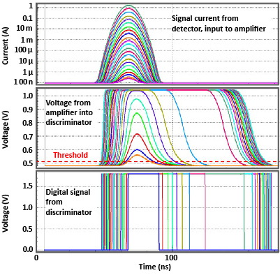
Figure 7: Circuit simulations of signal output from the APD (top), the output of the TIA (center), and the output from the threshold discriminator (bottom) for signals varying over greater than 90 dB.

The challenges for pulse-amplitude measurements caused by TIA saturation can be surmounted because, even when TIA output saturates, in this TIA design, the width of the output pulse increases with signal amplitude in a monotonic relationship, as shown in Figure 7, center. Accordingly, the lidar receiver’s comparator can be used to infer the pulse amplitude based on timing measurements of the rising and falling edges of the TIA output. The resulting time over threshold can be used as a surrogate for pulse amplitude in range-walk corrections. The calculation of the TOT digital pulse width and range walk (both in ns), measured from the simulations in Figure 7 are plotted as functions of pulse amplitude in Figure 8.

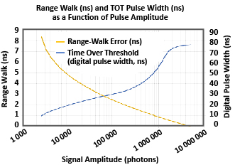
Figure 8: Simulation of range-walk error (primary y axis) and time over threshold (secondary y axis): The data plotted were measured for the various pulse amplitudes simulated in Figure 6.

While a lookup table can be used for range-walk correction for any receiver, piecewise linear or polynomial functional fits are effective in determining offset corrections. A sixth-order polynomial fit to the range-walk-offset error in Figure 8 is shown in Figure 9; also plotted is the residual error after the polynomial correction is subtracted from the pulse-amplitude data. The standard deviation of the residual-accuracy error is less than 8 mm.

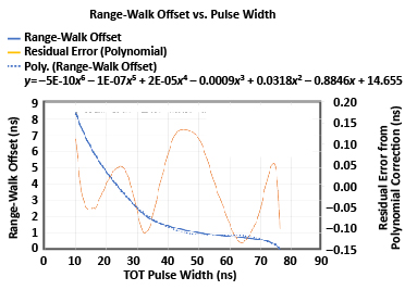
Figure 9: Simulation of residual range timing error: Residual range timing error (secondary y axis) resulting from simple piecewise linear correction of range walk plotted as a function of signal amplitude, compared to the original time walk (ns) measured. The standard deviation on the error corresponds to a range error of approximately 3 cm

The preceding examples were generated using simulated data. In practical applications, laser pulse shapes are not Gaussian. Passively Q-switched lasers, for example, often emit laser light for many tens of ns before the main laser pulse is emitted. This points to the importance of empirical calibration of any given lidar system design’s TOT characteristic based on application-specific requirements.

Field data taken on three identically configured time-of-flight sensors, configured with an Allegro 23 MHz APD photoreceiver and an Allegro 300 µJ passive Q-switched diode-pumped solid-state laser are shown in Figure 10. The data were taken at various ranges using targets of varying reflectivity. A fifth-order polynomial fit to the data is shown. The residual range error after the polynomial correction is applied to the data is shown in Figure 11. After using the same polynomial function to correct the data from three ranging systems, the standard deviation of the range data is less than 0.2 meters at all range distances. Our analysis suggests that much of the residual range error is due to the precision of the range measurements and jitter on the passive Q-switched lasers.

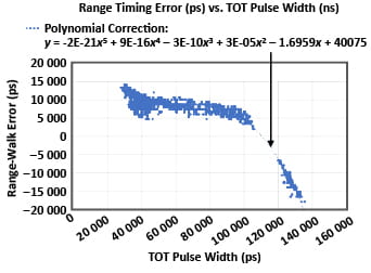
Figure 10: Error (in picoseconds) in range measurement as a function of the TOT pulse width extracted from range-measurement data taken over multiple ranges.

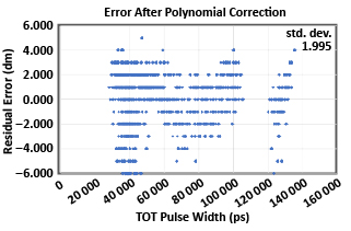
Figure 11: Residual error (in decimeters) as a function of measured TOT pulse width after polynomial correction. 

Conclusion

Leading-edge pulse detectors used in lidar systems are subject to both random and systematic errors, which result in loss of range precision and accuracy, respectively. While range precision can generally only be improved by increasing the return pulse amplitude or by averaging multiple pulses, the systematic amplitude-dependent error called range walk can be reduced in range measurements. Two techniques for correcting the systematic range-walk errors have been presented.

Time-variable threshold is shown to reduce the variation in the ratio between the return-pulse signal amplitude and the threshold level as a function of range, and thus to reduce the lidar susceptibility to return pulse amplitude variations. However, the technique is limited in dynamic range and is susceptible to target size, shape, and reflectivity variations, as well as atmospheric effects.

In contrast, time-over-threshold calibration, used with a fixed threshold or used simultaneously with time-variable threshold, allows for a reduction in systematic range-walk errors.

The simulated data presented here from Allegro’s APD photoreceiver have been used to demonstrate that systematic error is a monotonic function of TOT and to demonstrate the principals behind TOT calibration. Data obtained from field measurements presented here have demonstrated the ability to correct range-amplitude-dependent walk errors over 35 ns (greater than 10 meters) to within 0.2 meters of the true range values. 

 

^[1] The word precision is used to describe random error such as timing jitter. Here, we use accuracy to refer to systematic error such as range walk, which is the most common usage of the term. In the usage here, precision and accuracy are independent, so that any combination of high or low precision or accuracy is possible. An alternate use of the term accuracy, established by the International Organization for Standardization, encompasses both random and systematic error relative to the true value.

^[2] Non-two-dimensional targets can have other signal relationships. For example, wires can have an exp(–2σR) R^–3 signal variation as a function of range.