Lidar Effective Range

Introduction

The effective range of a lidar system depends on the sensitivity of its photoreceiver and the strength of optical signal returns as a function of target range. Parameters affecting signal-return strength are reviewed, including laser pulse energy, atmospheric conditions, and size, orientation, and surface properties of the target.

Lidar Overview

Since the introduction of lasers, light detection and ranging has proven to be one of the most useful methods to measure distance. Time-of-flight (TOF) lidar technology employs a method analogous to early radar that uses short pulses of light instead of microwaves. A TOF lidar system includes a laser transmitter that emits nanosecond-scale pulses, a photoreceiver circuit that detects and times optical pulses, and the optics required to project the laser onto a target, collect the back-scattered light, and focus it onto the photoreceiver. The round-trip time of flight (τ) between the transmission of an outgoing laser pulse and the arrival at the receiver of the pulse reflected by the target are used to calculate the target range (R) based on the speed of light in vacuum (c) and the average group refractive index of the optical path between lidar system and target (n):

Equation 1:

R = (c/2n)τ [m].

Lidar systems have limited effective range because the back-scattered optical signal weakens with target range, such that returns from very distant targets are too weak for the photoreceiver to detect. The effective range of a lidar system therefore depends on the sensitivity of its photoreceiver and the strength of optical signal returns as a function of target range.

Example Case:

To compare the effects of various parameters on lidar range performance, the example case summarized in Table 1 is, unless otherwise noted, used for cases presented throughout this paper. Also throughout this paper: an overfilled (OF) target is a target of a given cross-sectional area (usually 2.3 × 2.3 m²) at a range for which the projected laser spot is larger than the target; and an underfilled (UF) target is either an extended target such as a hillside or a target of specified cross-sectional area at a range for which the projected laser spot is smaller than the target.

Table 1: Parameters for Example Case

Parameter	Description	Value
At	Target cross-sectional area	2.3 x 2.3 m2
ϕ	Half-angle laser beam divergence	0.5 mrad
ROF	Range beyond which a target becomes overfilled	2.6 km
Etx	Transmitted laser pulse energy	300 μJ
θ	Angle of incidence	30°
ρ	Diffuse reflectivity	30%
η	Efficiency of the optical system	90%
D	Receive-aperture diameter	21mm
Nf	Factor required to achieve a particular FAR	8
NEI	Noise equivalent input	33 ph
λ	Laser wavelength	1534 nm
EPh	Photon energy (in Joules)	1.28 x 10-19 J

Radiometric Model

The signal-return level that determines the effective range of a lidar system depends on the photoreceiver’s sensitivity and the maximum false-alarm rate (FAR) tolerated by the application. Lidar systems are designed to ignore pulses weaker than a specified detection threshold in order to extinguish false alarms caused by photoreceiver noise, but optical signal returns that are weaker than the detection threshold are also ignored. Accordingly, lidar systems are operated with the minimum detection threshold required to achieve a FAR just below the maximum permitted by the application. Detection thresholds are frequently 6 to 10 times the receiver noise.

For average signal levels equal to the detection threshold, the probability of detection (P_d) averaged over an ensemble of identically prepared pulses is 50%. Detection probability increases for signal levels that exceed the detection threshold according to the complementary cumulative distribution function (CCDF) of the photoreceiver’s output. However, the trends of P_d and FAR with detection threshold depend on details internal to the photoreceiver. A general analysis of lidar effective range can proceed from understanding that the detection threshold is a fixed multiple of the photoreceiver sensitivity, likely 6 to 10, and that signals at the detection threshold will be detected with 50% probability.

Photoreceiver sensitivity can be quantified in terms of the notional optical signal level at the photoreceiver input that will result in an average output level equal to the magnitude of the photoreceiver output noise. When the notional optical-signal level is measured in units of power, sensitivity is quantified by a noise-equivalent power (NEP); if the signal level is expressed in units of photons, then a noise-equivalent input (NEI) may be specified. Photoreceiver sensitivity is a function of laser pulse width, detector operating temperature, and, for avalanche photodiode (APD)-based receivers, the avalanche gain of the APD.

With receiver noise expressed as an equivalent signal level, the threshold signal level (S_th) that determines lidar effective range can be expressed as either:

Equation 2:

S_{th_NEP} = N_f × NEP [W]; or

Equation 3:

S_{th_NEP} = N_f × NEI [photons],

where N_f is the factor required to achieve a particular FAR requirement, usually in the range of 6 to 10.

Given S_th, a radiometric model can be used to determine the average reflected signal amplitude received by a lidar system under specific conditions and against a particular target. The combination of the radiometric model and S_th result in the range equation, which gives the effective range of a lidar system based on the characteristics of the transmitted laser pulse, the target, and the intervening atmosphere.

Laser pulses are attenuated as they propagate through the atmosphere and may be broadened, defocused, and even deflected from straight-line paths by local refractive-index variations caused by changes in atmospheric density that evolve over time due to wind and turbulence. The pulse is attenuated and distorted to an extent that depends on the wavelength and power of the laser, the length of the optical path through the atmosphere, and the characteristics of the atmosphere, such as temperature, visibility, and turbulence intensity.

The combined effects of absorption and scattering can be characterized by the optical power (or pulse energy) attenuation coefficient (σ) in units of m^–1. The laser fluence within the cross-sectional area of the beam (A_beam) in m², at range R in meters, can be approximated as:

Equation 4:

F = (E_tx/A_beam) exp(–σR) = [E_tx/π(ϕR)²] exp(–σR) [J m^–2],

where E_tx is the transmitted laser pulse energy in Joules, and ϕ is the half-angle laser beam divergence in radians.

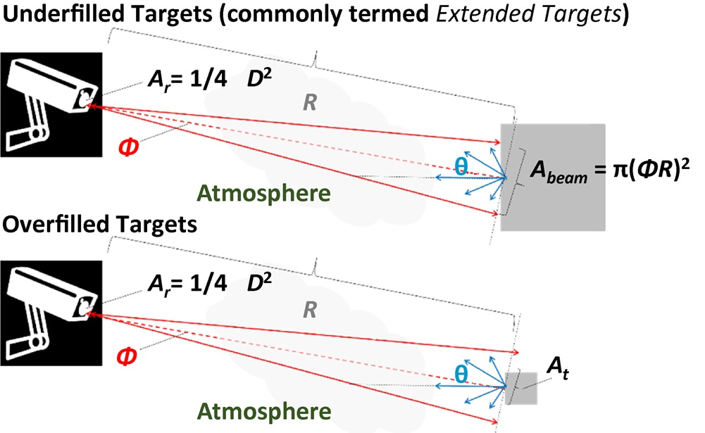
Depending on the beam divergence, the size of the target, and the range to the target, a laser spot projected onto a target may either: underfill the target (Figure 1, top), in which case all of the energy in the laser pulse is scattered by the target; or overfill the target (Figure 1, bottom), in which case only a portion of the pulse energy will be scattered by the target. In either case, if the laser beam strikes the target surface at angle of incidence θ, the fluence into the target surface is reduced by a factor of cos(θ) because the laser spot projected onto the tilted surface elongates by 1/cos(θ). However, this only impacts the total energy incident on the target (G_ti) in the overfilled case. 

 

Ar	Cross-sectional area of the receive aperture in m2
D	Receive aperture diameter in meters
R	Range to target in meters
Abeam	Cross-sectional area of the beam in m2
Φ	Half-angle laser beam divergence in radians
θ	Angle of incidence in radians
At	Target cross-sectional area in m2

Figure 1: Ranging of an underfilled target (larger than the laser spot; top) and an overfilled target (smaller than the laser spot; bottom)

For an underfilled target (commonly termed an extended target; see Figure 1, top), energy incident on the target is:

Equation 5:

G_{ti_UF} = E_tx exp(–σR) [J].

The factor of cos(θ) related to laser angle of incidence does not appear in Equation 5 because the change in laser spot size cancels with the change in fluence. This can be considered another way: If the laser spot is contained within the target area, then 100% of the energy in the laser pulse must be delivered to an underfilled target surface.

For an overfilled target (Figure 1, bottom), incident energy is the product of the reduced fluence and the target area (A_t, in m²):

Equation 6:

G_{ti_OF} = A_t cos(θ)[E_tx/π(ϕR)²] exp(–σR) [J].

Another way to think about the cos(θ) factor in Equation 6 is that the fraction of the laser pulse energy intercepted by an overfilled target is the ratio of the area of the target projection onto a plane normal to the laser beam, and the laser spot area in that plane. The target area projected onto a beam-normal plane shrinks as cos(θ).

Equation 6 does not automatically ensure that the target is overfilled, and spurious results will be obtained from Equation 6 if the target area is larger than π(ϕR)². Likewise, Equation 5 will give the wrong result for an overfilled target. To determine the correct equation to apply, the target must be modeled and determined to be underfilled or overfilled at a given range. Although the incident laser pulse energy depends on the detailed shape and aspect presented by a target object—as well as the aiming accuracy of the lidar system—the range beyond which a target becomes overfilled can be approximated as:

Equation 7:

 

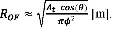
The factor of cos(θ) in Equation 7 accounts for the change of the target cross section in the laser beam, modeled as a single planar surface tilted relative to the beam axis. However, it should be remembered that a real three-dimensional target object has other surfaces that will rotate into the beam as other surfaces rotate out of the beam. (Methods to account for multiple target surfaces and orientations are discussed later.)

If the target is a Lambertian reflector characterized by a diffuse reflectivity (ρ), the total reflected energy (G_tr) is:

Equation 8:

G_tr = ρG_ti [J],

where G_ti is either G_{ti_UF} or G_{ti_OF} as appropriate. Reflected energy per unit solid angle varies with direction as:

Equation 9:

G_tr,Ω = [(ρG_ti)/π] cos(θ′) [J sr^–1],

where θ’ is angle of reflection relative to the target surface normal.

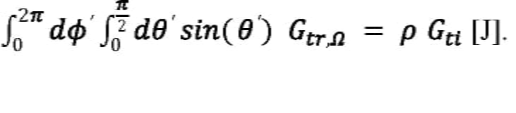
Note that π—rather than 2π—appears in the denominator of Equation 9 because of the cos(θ’) directional factor. If the differential surface element—sin(θ´) dθ´ dϕ´ in spherical polar coordinates, where θ´ is the zenith angle and ϕ is the azimuth angle—is integrated over a unit hemisphere, the area of the hemisphere (2π) results. However, if the differential surface element is multiplied by cos(θ´), π results. Thus, if G_tr,Ω is integrated over a unit hemisphere, the total reflected energy (G_tr = ρG_ti) is recovered, as expected:

Equation 10:

 

The reflected energy per unit solid angle radiated in the direction of the lidar system is found by setting θ´ equal to θ in Equation 9. After factoring in atmospheric attenuation, the energy reflected into the lidar system receive aperture is the product of Gtr,Ω and the solid angle subtended by the receive aperture (Ωrx), which is:

Equation 11:

Ω_rx = (πD²)/(4R²) [sr],

where D is the diameter of the receive aperture in meters.

The reflected laser pulse energy delivered to the photoreceiver detector is therefore:

Equation 12:

E_rx = ηG_tr,Ω Ω_rx exp(–σR) [J],

where η is the efficiency of the optical system.

If E_rx is written explicitly for the underfilled and overfilled cases, an R2 dependence (neglecting attenuation) is found for underfilled targets:

Equation 13:

E_{rx_UF} = ηρE_tx cos(θ) D² [exp(–2σR)]/(4R²) [J];

And an R4 dependence is found for overfilled targets:

Equation 14:

E_{rx_OF} = ηρE_tx A_t cos²(θ) D² [exp(–2σR)]/(4πϕ²R⁴) [J],

where Equation 13 applies if R is less than R_OF, and Equation 14 applies if R is greater than R_OF.

In Equation 13 and Equation 14, it may be counter-intuitive— when considering that Lambertian reflection normally results in isotropic radiance—to retain the factor of cos(θ) associated with Equation 8. In passive-imaging applications where the entire scene is illuminated by ambient light or emits blackbody radiation and the target spans the instantaneous field of view of a detector pixel, the radiating surface area within the instantaneous field of view varies as 1/cos(θ), canceling the cos(θ) associated with Lambertian reflection. This is similar to how cos(θ) factors cancel in Equation 5 for the energy incident on an underfilled target surface, with the exception that, in that case, the cos(θ) factor that affects fluence into the target results from illumination of the target with a collimated beam transmitted from the lidar system, prior to reflection. Thus, for a lidar system, there are separate factors of cos(θ) that account for directional illumination and Lambertian reflection and, in the underfilled case, only one factor of cos(θ) cancels due to elongation of the laser spot on the target; for the overfilled case, cancelation does not occur because the radiating surface area is limited by the physical size of the target.

A threshold-signal level from Equation 3 expressed as a multiple of the photoreceiver NEI in units of photons can be multiplied by the photon energy in Joules (E_ph) to arrive at a threshold value of:

Equation 15:

E_{rx_th} = N_f × NEI × E_ph [J],

where:

Equation 16:

E_ph = (1.9864 × 10^–16)/λ [J],

where the numerator is expressed in J nm, and λ is the laser wavelength in nm.

Alternatively, if photoreceiver sensitivity to laser pulses of a particular width (T_p in seconds) is expressed as NEP, the threshold value of E_rx can be approximated for square laser pulses as:

Equation 17:

E_{rx_th} ≈ Nf × NEP × T_p [J].

The maximum effective range (R_max) of a lidar system against underfilled or overfilled targets can be found by equating Equation 13 or Equation 14, respectively, to E_{rx_th} and solving for R. However, the occurrence of R in the atmospheric attenuation factor exp(–2σR) as well as in the R² and R⁴ denominator terms of Equation 13 and Equation 14 prevent solution in terms of elementary functions. In the limit of negligible attenuation, assuming receiver sensitivity expressed as NEI, maximum effective range for an underfilled target is:

Equation 18:

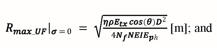
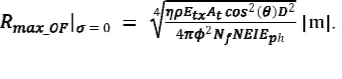
Maximum effective range for an overfilled target is:

Equation 19:

 

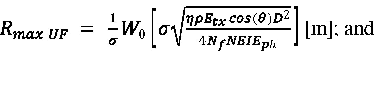
If atmospheric attenuation is included in the calculation, the solutions involve the principal branch of the Lambert W function, W0[x exp(x)] = x for W ≥ –1. This special function is computed numerically by mathematical software packages such as MATLAB (where the function is called lambertw) and Mathematica (where the function is called ProductLog). The general solution for the underfilled target case is:

Equation 20:

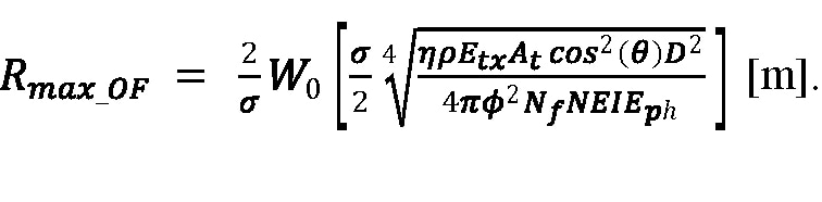
The general solution for the overfilled target case is:

Equation 21:

Equation 18, Equation 19, Equation 20, and Equation 21 must be used with caution because whether a target is underfilled or overfilled depends on its range. A maximum effective range computed for the underfilled case using Equation 18 or Equation 20 may result in a value of R_max for which a target is overfilled, which would therefore be invalid. Similarly, a calculation using Equation 19 or Equation 21 based on the assumption that a target is overfilled may find a maximum effective range for which the target is actually underfilled. It is therefore necessary to compare R_max to ROF in order to validate results from Equation 18, Equation 19, Equation 20, and Equation 21. Using the example case, effective range is calculated in Figure 2 as a function of various atmospheric attenuation coefficients corresponding to conditions from visible through light fog. (These conditions and more-limited-visibility conditions are discussed further in the "Atmospheric Conditions" section.)

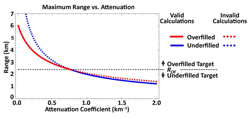
Figure 2: Maximum effective range for overfilled and underfilled cases vs. atmospheric attenuation coefficient. (Overfilled and underfilled data are solid where applicable and dashed in the range where they do not apply.)

Laser Pulse Energy and Receive Aperture

The energy delivered to a lidar system detector (E_rx, expressed in photons) is plotted in Figure 3 for various transmitted pulse energies for an atmospheric attenuation coefficient of σ = 0.05 km^–1, which corresponds to 23 km visibility. Horizontal dashed lines mark detection thresholds corresponding to S_th = 3 × NEI and 8 × NEI. The intersection of an E_rx curve with the S_th line is another way to find the maximum effective range. Oblong targets become overfilled along their short axis at a closer range than the point at which the laser spot is wider than their long axis, such that the fraction of the laser spot intercepted by a partially overfilled target varies with range; in that case, the closed-form expressions for effective range given by Equation 20 and Equation 21 do not apply, and R_max must be found graphically, as in Figure 3, or by using a numerical solver. 

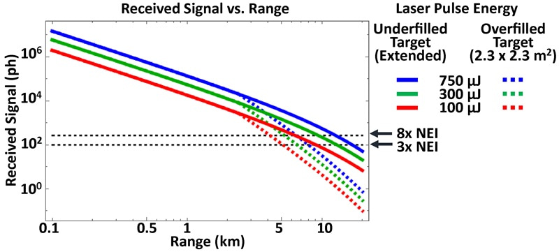
Figure 3: Received signal vs. range for various transmitted pulse energies, against underfilled and overfilled targets.

Effective ranges for different combinations of transmitted pulse energy, detection threshold, and receive aperture are summarized in Figure 4 for underfilled and overfilled targets. An atmospheric attenuation coefficient of σ = 0.05 km^–1 is assumed. 

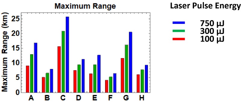
Lidar and Target Parameters for Effective Ranges Charted

Sth = 3 x NEI				Sth = 8 x NEI
D = 21 mm		D = 50 mm		D = 21 mm		D = 50 mm
UF	OF	UF	OF	UF	OF	UF	OF
A	B	C	D	E	F	G	H

OF = Overfilled target (target is 2.3 x 2.3 m²)

  UF = Underfilled target (target is extended; i.e., larger than beam width)

Figure 4: Maximum range for the lidar and target configurations summarized for various transmitted pulse energies.

Target Reflectivity

The laser energy that reaches a target surface is partially absorbed and partially reflected. The energy reflected from the target is the sum of a diffuse component that scatters in all directions (Figure 5, top) and a specular component directed along an angle of reflection equal to the angle of incidence but in the opposite direction from the surface normal (Figure 5, bottom, longest outgoing ray). Obviously, the absorbed portion of the laser pulse energy cannot contribute to signal at the lidar receiver. Moreover, because the photoreceiver of a lidar system is collocated with its laser transmitter, pure specular reflections only reach the receiver in the unusual circumstance of perfectly normal incidence or the special case of a retroreflective target; that is the main reason lidar calculations usually assume diffuse reflection.

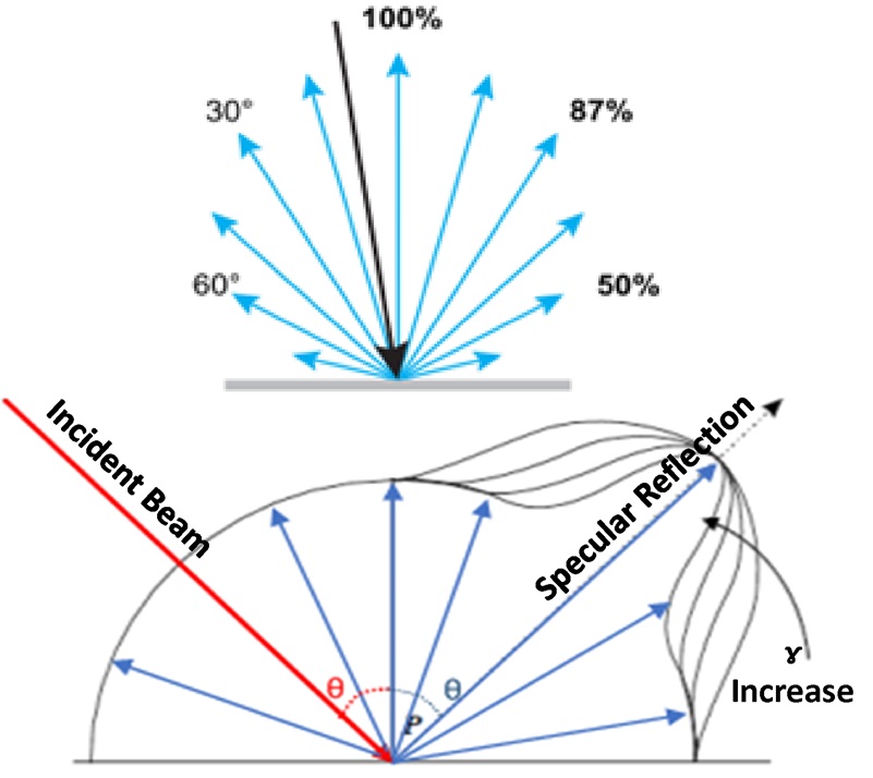
Figure 5: Diffuse reflector (top) and reflection geometry with diffuse and specular components (bottom), where ɣ is the specular reflectivity index.

The cosine dependence of diffuse reflection was previously given in Equation 9, expressed in terms of reflected energy per unit solid angle. This is a version of the Lambert cosine law, which is more commonly expressed in terms of radiant intensity (I_e,Ω) in units of W sr^–1. The cosine law for radiant intensity is Equation 9 divided by the laser pulse width, which converts the total energy delivered by a laser pulse to the average power of the pulse.

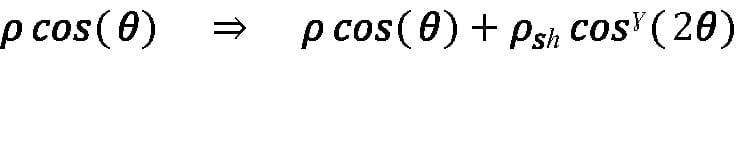
Assuming perfect Lambertian reflection simplifies Equation 20 and Equation 21, but most targets depart from the ideal model. Often, reflectivity increases near the angle of specular reflection. This characteristic is referred to as a specular highlight because of its directional dependence, but unlike a pure specular reflection, reflectivity is enhanced at angles in the vicinity of the angle of specular reflection, and not just at the exact angle of specular reflection. A phenomenological model developed by B. T. Phong in 1975 for use in computer graphics represents specular highlights by replacing the product ρ cos(θ’) in Equation 9 with:

Equation 22:

 

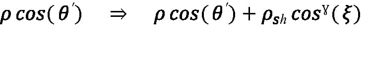
where ρ is the diffuse reflectivity introduced earlier, θ’ is the angle between the reflected ray and the target surface normal, ρ_sh is a specular highlight reflectivity coefficient, ξ is the angle between the reflected ray and the direction of pure specular reflection, and ɣ is a shape parameter that affects the angular width of the specular highlight. The effect of shape on the magnitude of the total reflectivity can be observed in Figure 5, bottom, where increasing ɣ narrows the specular highlight feature.

The substitution of Equation 22 carries through to Equation 20 and Equation 21, where—for a lidar system—the angle of the back-reflected ray to the lidar system receiver is the same as the laser angle of incidence on the target surface, which results in θ’ = θ. The angle between back-reflected ray and the direction of pure specular reflection is ξ = 2θ, because the angle of specular reflection is equal to the angle of incidence, but in the opposite direction from the surface normal. Accordingly, Equation 20 and Equation 21 can incorporate the Phong model by making the substitution:

Equation 23:

 

Ranging of target surfaces in the vicinity of normal incidence is a more common occurrence than perfectly normal incidence, so enhanced reflectivity caused by specular highlights can be relevant to lidar performance. However, because the Phong model is phenomenological rather than based on first principles, there is no general theory by which ρsh and ɣ can be calculated from fundamental material and surface properties. Moreover, analytic models such as Equation 20 and Equation 21 are primarily useful because of their clarity and ease of use. Given the variety of real-world target surfaces and orientations, refinements such as Equation 23 increase model complexity without necessarily improving model accuracy. Indeed, analytic models such as Equation 20 and Equation 21 are most useful when applied to bound system performance by considering the least-favorable set of target assumptions under which the lidar system must function, as well as the average case. The possible enhancement of target reflectivity by nearly normal incidence is usually not the worst-case scenario, and—for the average case—it is simpler to lump the average enhancement of reflectivity by specular highlights into an average diffuse reflectivity than to explicitly apply Equation 23.

Because ρ is paired with E_tx in Equation 20 and Equation 21, variations of ρ with fixed transmitted laser pulse energy are equivalent to variations of transmitted laser pulse energy for fixed ρ. Consequently, the variation in maximum effective range shown in Figure 4 for the three transmitted laser pulse energies of 100 μJ, 300 μJ, and 750 μJ against the example case of a 30% reflective target also correspond to the range performance with a fixed laser energy of 250 μJ and target reflectivities of 12%, 36%, and 90%. In general, everything in the numerator under the radical in Equation 20 and Equation 21—laser pulse energy, target reflectivity, receiver aperture area, and the cosine orientation factor—trades proportionally with one another and has the same impact on effective range. Maximum effective range is plotted in Figure 6 for the example case target as a function of reflectivity for various atmospheric attenuation coefficients.

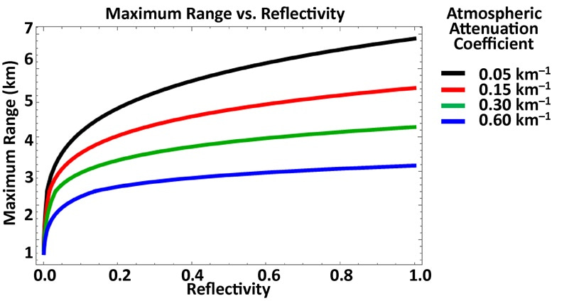
Figure 6: Maximum effective range vs. reflectivity coefficient for various atmospheric attenuation coefficients.

Angular Orientation

Maximum effective range is plotted versus angle of incidence in Figure 7 for various atmospheric attenuation coefficients, calculated using Equation 20 and Equation 21 and reflecting the different θ dependence of the underfilled and overfilled cases, respectively. As with target reflectivity and the phenomenon of specular highlights, it is usually more useful to analyze least-favorable and average cases of target surface orientation than to construct more-complex analytic models. The 50.5-degree case results in the average cosine factor obtained for a composite target comprising an ensemble of smaller surfaces of orientation uniformly distributed between θ = 0 degrees and θ = 90 degrees.

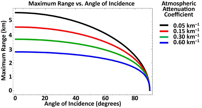
Figure 7: Maximum effective range vs. angle of incidence for various atmospheric attenuation coefficients.

Target Shape

Real-world target objects present multiple surfaces of varying area characterized by reflectivities and angles of orientation that depend on the aspect from which the target is regarded. Irregularly shaped targets become overfilled along short cross-sectional axes at closer range than along longer axes, and targets such as trees may be perforated by holes through which laser energy can pass without contributing to the reflected signal. Accordingly, analytic models of maximum effective range based on a single target surface of regular shape, such as Equation 20 and Equation 21, are helpful for understanding the physical dependencies of lidar performance but cannot produce universally applicable results. Numerical calculations based on detailed three-dimensional target models can be used for specific applications, but one way to represent target complexity in an analytic model is to consider a target composed of multiple smaller target surfaces. Lidar performance against a typical complex target is then estimated based on averages of surface reflectivity and angles of incidence. When this is done, rather than finding separate values of E_rx for each component surface, it is practical to reduce the average reflectivity by an average cosine factor. The neutral assumption that angles of incidence are uniformly distributed between 0 and π/2 results in an average cosine factor of 2/π ≈ 0.637, which can replace cos(θ) in Equation 20 and Equation 21. Alternatively, θ = arccos(π/2) ≈ 50.46 degrees can be used directly in Equation 20 and Equation 21.

Atmospheric Conditions

Atmospheric attenuation results from scattering and absorption by molecules and aerosols. The total atmospheric attenuation coefficient is the sum of coefficients for the individual processes:

Equation 24:

σ = α_m + β_m + α_a + β_a [m^_–1],

where α is an absorption coefficient and β is a scattering coefficient, and the subscripts m and a designate the molecular and aerosol processes, respectively.

The molecular and aerosol absorption processes in the short-wavelength infrared result from vibrational excitation of the molecules from which the atmosphere and suspended particles are composed. Molecular scattering is another term for Rayleigh scattering, whereas aerosol particles of size comparable to the optical wavelength scatter light by the Mie process; much larger particles as well as fluctuations of the refractive index along the optical path, due to changes in atmospheric density, scatter light according to the rules of optics. The absorption processes are very wavelength-selective and depend on the specific molecular species present: Whereas Rayleigh scattering drops as 1/λ⁴, Mie and geometric scattering intensity do not depend very strongly on wavelength.

Attenuation coefficients for various atmospheric conditions are shown in Table 2 in units of km^–1. Note that these values must be converted to m^–1 for use in the equations of this paper, which are written in terms of SI units.

Table 2: Attenuation Coefficients: Various Atmospheric Conditions

Attenuation Coefficient	km-1 (1534 nm)
Heavy fog (0.05 km visibility)	62.6
Rain	10
Light fog	1.00
Moderate fog (0.25 km visibility)	9.71
Hogg fog (1km visibility)	2.07
4 km visibility	4.61 x10-01
Maritime haze	7.40 x 10-02
Haze	1.50 x 10-02
10 km visibility	9.21 x 10-02
23 km visibility	4.61 x 10-02
Pure air	1.00 x 10-02

Sunlight

Because a lidar system only needs to respond to the transmitted laser wavelength, lidar systems generally have a narrow-passband filter on the receive optics. Likewise, because a lidar system only needs a field of view that is wide enough for practical alignment to the projected laser spot, the view from a lidar system of the solar-illuminated background surrounding a target is fairly limited. These factors tend to minimize the impact of sunlight on a lidar system.

The atmospheric mass 1.5 solar spectral irradiance used for photovoltaic system design provides a good estimate for the solar background at ground level. At 1534 nm, the solar spectral irradiance at ground level is approximately E_e,λ = 0.26 W m^–2 nm^–1 after traveling 1.5 times the zenith path length through the atmosphere. Assuming the background is a Lambertian reflector characterized by ρ—neglecting atmospheric attenuation and efficiency losses in the optics— the flux on the lidar detector is:

Equation 25:

Φ_e = (π/16) E_e,λ Δλρω² D² [W],

where Δλ is the filter bandpass in nm, and ω is the lidar angular field of view in radians. For Δλ = 10 nm, ρ = 30%, ω = 10 mrad, and D = 50 mm, the flux on the detector is about 38 nW. The resulting background photocurrent is the product of Φ_e and the detector responsivity, which is about 1 A W^–1 for an InGaAs photodiode and M times greater for an InGaAs APD operating at avalanche gain M.

Background photocurrent has the same noise impact as the dark current of a detector; therefore, if the background photocurrent is of magnitude similar to the detector dark current, it may affect the sensitivity of an APD-based lidar system, depending on the gain operating point of the APD with respect to the noise of its amplifier circuit. Conversely, if background photocurrent is more than an order of magnitude less than the detector dark current, its impact on lidar sensitivity is negligible. Likewise, neither dark current nor background photocurrent typically affect the sensitivity of photodiode-based lidar circuits, which—being less sensitive than APD-based lidar systems—are dominated by amplifier noise.

When ranging targets at a small angular separation from the solar disk, increased background photocurrent from the received sunlight can potentially increase the FAR at a fixed detection threshold. Calculating the impact of background photocurrent on a lidar system requires the analytic methods previously discussed. In general, however, if shot noise on background photocurrent becomes significant, the detection threshold of a lidar system must be increased to reduce the FAR; thus, S_th must increase, reducing the maximum effective range of the lidar system.

Refractive Index Variations

Because range is calculated based on the speed of an optical pulse traversing the path between the lidar system and the target, range accuracy depends on knowing the average group refractive index of the atmosphere in that path, which depends on the refractive index of the atmosphere and its dispersion near the laser wavelength. The group velocity of an optical pulse traveling in vacuum is the same as its phase velocity, c = 299,792,458 m s^–1; and, for a laser pulse traveling through some medium like air, this speed is reduced by the group refractive index. General models for the refractive index of air calculated as a function of wavelength, air temperature, atmospheric pressure, humidity, and carbon dioxide content have been published, two of which have been implemented by NIST as web-based calculators.^[1]

The refractive index of air—at 20°C under average sea-level pressure, at 50% relative humidity, with 450 ppm CO₂ partial pressure—is 1.000268148. This value can be used for baseline calculations. However, because the time of flight for laser pulses depends on the average propagation speed along the optical path, the accuracy of longer-distance measurements is affected by uncorrected group refractive-index errors. An uncorrected average-refractive-index error (Δn) results in a range-measurement error (ΔR) that is proportional to the actual range:

Equation 26:

ΔR = Δn R [m].

Small environmental changes—like a 1-degree Celsius change in temperature or a 0.4 kPa change in air pressure— can result in refractive index changes as great as one part per million.

Last, as suggested in the "Atmospheric Conditions" section, spatial fluctuations of the refractive index along the optical path between the lidar system and the target can scatter and redirect propagating laser pulses. In addition to contributing to attenuation, these refractive-index fluctuations can guide laser pulses off the straight-line path between lidar system and target, affecting the range measurement. As with range error, the severity of attenuation and distortion increases with target range. 

^[1] See https://emtoolbox.nist.gov/Wavelength/Abstract.asp; accessed November 8, 2018